
Earthquakes are a complicated spatio-temporal phenomenon. The number of earthquakes with a magnitude M>m is given by the Gutenberg-Richter law. In addition to the regularity in the rate of occurrence, earthquakes display a complex spatio-temporal behavior. The spatial distribution of epicentres is fractal and they occur on a fractal-like structure of faults. Short-range temporal correlations between earthquakes are expressed by Omori's law, which states that immediately following a main earthquake there is a sequence of aftershocks whose frequency decays with time as T-a, a = 1. This has led to the commonly held belief that aftershocks are caused by a different relaxation mechanism than the main shocks.
The observed temporal complex behavior is obviously of dynamical origin. However, the statistics of earthquakes as well as the geometrical fractal structure displayed by the faults and by the spatial distribution of epicenters is also a result of a dynamical process and one might speculate whether it is possible to unify these observations.
We show that the distribution of waiting times between earthquakes occurring in California obeys a simple unified scaling law valid from tens of seconds to tens of years. The short time clustering, commonly referred to as aftershocks, is nothing but the short time limit of the general hierarchical properties of earthquakes. There is no unique operational way of distinguishing between main shocks and aftershocks. In the unified law, the Gutenberg-Richter b-value, the exponent -1 of the Omori law for aftershocks, and the fractal dimension df of earthquakes appear as critical indices.
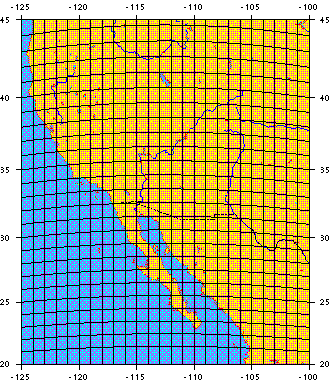
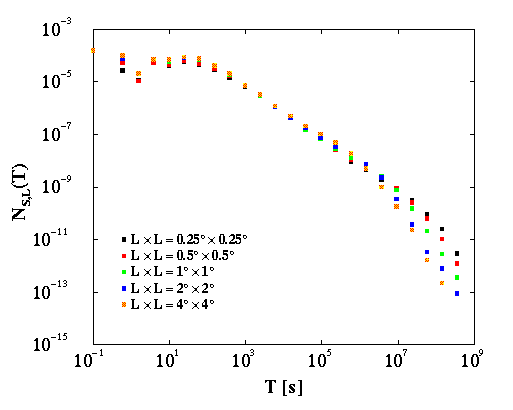
The spatio-temporal analysis was carried out as follows. We covered the region with a grid with cells of size LxL, see Figure 1, and defined the waiting time T as the time interval between the beginning of two successive earthquakes. We then measured NS,L(T), the distribution of waiting times T, between earthquakes occurring within range L whose magnitudes are greater than m = Log10(S).


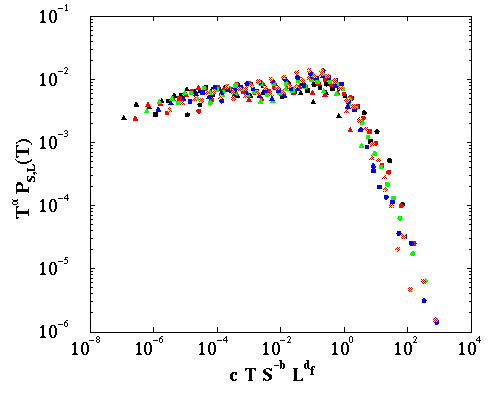
The function f(x) consists of a constant part and a decaying part, separated by a sharp kink. The constant part corresponds to the linear, power-law part since we have multiplied NS,L(T) with Ta. Any deviation from power-law behavior would show up dramatically in this type of plot. Nevertheless, the function is approximately constant over 8 orders of magnitude! The rapidly decaying part is consistent with an exponential decaying function implying an uncorrelated regime for large values of x. This is indeed what one would expect on physical ground: earthquakes that are separated by large enough distances or long waiting times will be uncorrelated.
The index a = 1 can be identified as the Omori-law exponent for aftershocks, b = 1 is the b-value in the Gutenberg-Richter law, and df = 1.2 describes the 2d fractal dimension of the location of epi-centers projected onto the surface of the Earth.
The data collapse implies that the waiting time distribution depends on T, S, and L only through the variable $x$. Only critical processes exhibit this type of data collapse, known as scaling in critical phenomena, so our analysis demonstrates that earthquakes are a self-organized critical (SOC) phenomenon, as had been anticipated from the existence of the Gutenberg-Richter law. The data collapse shows that there is no separate relaxation mechanism for aftershocks.
Depending on the value of scaling argument x, and thus the chosen values of L and m (or S), two successive earthquakes will either be correlated, for x small, (i.e. to the left of the kink in Fig. 4, or uncorrelated, for x large (i.e. to the right of the kink in Fig. 4.
Depending on the length scale L of observations, and the magnitude magnitude m (or S) chosen, the correlated Omori Ta regime may range from seconds to tens of years (and probably much longer if data were available). If the earthquakes are correlated they may be interpreted as belonging to an aftershock sequence. If they are uncorrelated, they may be interpreted as main events. However, this depends on L and m through the variable x and has no absolute meaning. Therefore, there is no unique way of characterizing earthquakes as aftershocks or main events.
To summarize, the short time correlations given by Omori's law is just the short time limit of a general hierarchical scaling phenomenon occurring at all accessible time scales. Amazingly, the statistics of aftershocks occurring within minutes of an earthquake can be simply related to the statistics of earthquakes separated by tens of years!
How should one physically understand the fundamental unified scaling law
Think of earthquakes being generated by 'processes', each producing a sequence of correlated earthquakes with a Ta distribution. These processes correspond to a sequence of avalanches in self-organized critical models of complex phenomena. Visually, one might think of the processes as the activity associated with dynamically changing fault segment patterns. The law indicates that the crust operates in the true SOC slow-driving regime where the individual processes (avalanches) do not overlap. Because of the non-zero driving rate, several spatially separated processes are active simultaneously. The kink on the f-curve indicates the point where one crosses into the regime where spatially independent earthquakes, belonging to different processes, are sampled within a window spanned by T and L. For small enough L and T only a single, correlated process is sampled.
PUBLICATIONS