Our calculations of the conductance, described below, require detailed structural information about the quantum wire. A direct way of describing such a system would be by providing detailed geometric and structural information about an actual wire. Such data can be represented in a convenient form as a set of probability distributions and correlation functions of some basic parameters of the wire (e.g. the width, width fluctuations, confining potential etc). The detailed structure can be recovered, in a statistical sense, by generating wires using an appropriate algorithm and the set of probability distributions and correlation functions as an input. In order to examine the electronic properties of some realistic structures we have used structural information obtained in the Monte-Carlo simulation of vicinal surface grown quantum well wires by Hugill et al. (1989).

Figure 1: Plot of a section of the generated (real) quantum wire of average
width 10, with island concentration p=0.05.
Quantum wires directly grown by epitaxial growth of a heterostructure,
usually (Al,Ga)As, by using more or less controlled generation of
terraces and steps (or corrugations) on semiconductor surfaces, seemed
very attractive (Petroff et al. 1984, Fukui and Saito 1987, Miller et al. 1992, Nötze et al. 1991).
This process was at one time considered very promising for the
eventual realization of very narrow (about a few nanometers)
quantum wires![]() . More recently attention has shifted to other
possibilities, such as V-grooves, but as the basic principles governing the
electronic structure are common to different sorts of wires we shall
concentrate here on MBE grown wires.
The kinetics of MBE can be successfully simulated on a computer
(Hugill et al. 1989, Joyce et al. 1990), provided that the values of the model parameters are
correctly estimated from the experimental data. This enables one to perform
Monte Carlo simulations of these wire structures and therefore, to
define structural disorder in the system (Taylor et al. 1991, Nikolic and MacKinnon 1993).
A section of a generated monolayer wire with an average width of 10 lattice
sites is shown in Fig. 1. The effects of the various types of
compositional disorder considered here have implications for the
electronic behaviour of quantum wires fabricated by other techniques.
. More recently attention has shifted to other
possibilities, such as V-grooves, but as the basic principles governing the
electronic structure are common to different sorts of wires we shall
concentrate here on MBE grown wires.
The kinetics of MBE can be successfully simulated on a computer
(Hugill et al. 1989, Joyce et al. 1990), provided that the values of the model parameters are
correctly estimated from the experimental data. This enables one to perform
Monte Carlo simulations of these wire structures and therefore, to
define structural disorder in the system (Taylor et al. 1991, Nikolic and MacKinnon 1993).
A section of a generated monolayer wire with an average width of 10 lattice
sites is shown in Fig. 1. The effects of the various types of
compositional disorder considered here have implications for the
electronic behaviour of quantum wires fabricated by other techniques.
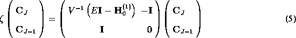
For the purpose of transport calculations the quantum wire is sandwiched between two perfect leads. The same model using a tight-binding, nearest-neighbour Hamiltonian is used to describe both the quantum wire and the leads:
where  is the localized `Wannier' state or atomic orbital on site
 ,
,  is the `site energy' and
  is the hopping
matrix element between sites and
is the hopping
matrix element between sites and  . We shall assume that is
zero unless the and sites are nearest neighbours, when
. We shall assume that is
zero unless the and sites are nearest neighbours, when
 (i.e.
(i.e.  defines our unit of energy and the effective mass).
We define our lead-sample-lead system to lie along the  -axis. It can be
divided into slices along that direction, each of which has
-axis. It can be
divided into slices along that direction, each of which has  sites (i.e. a
cross-section
of the quantum wire).
The elastic scattering in the quantum wire (which extends from
slice 1 to slice
sites (i.e. a
cross-section
of the quantum wire).
The elastic scattering in the quantum wire (which extends from
slice 1 to slice  )
is described by transmission probabilities
)
is described by transmission probabilities  , which describe
the probability that an electron incident in channel (state)
, which describe
the probability that an electron incident in channel (state)  on the left
emerges
in channel
on the left
emerges
in channel  on the right. The amplitude transmission coefficients
  can be calculated by various means. Here the formulation due to
Ando (1991) is used
can be calculated by various means. Here the formulation due to
Ando (1991) is used
where
and  is the longitudinal velocity in subband .
 is the Green's function which couples the
  th and the
 st
slice in our system (i.e. the last slice in the left-lead and the first slice
in
the right-lead).
The matrices
st
slice in our system (i.e. the last slice in the left-lead and the first slice
in
the right-lead).
The matrices
and
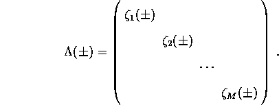
contain the eigenvectors and eigenvalues respectively of the eigenvalue problem
The perfect leads extend to
 and
and  along -axis. In these asymptotic regions
the incident and transmitted states obey the Schrödinger equation
along -axis. In these asymptotic regions
the incident and transmitted states obey the Schrödinger equation
where  is replaced by the Hamiltonian of an isolated
ordered slice
is replaced by the Hamiltonian of an isolated
ordered slice  .
.
 is a vector describing the amplitudes of the wavefunction on
the
is a vector describing the amplitudes of the wavefunction on
the  th slice.
The superscript designates the length of the system.
Although
th slice.
The superscript designates the length of the system.
Although  is generally a diagonal matrix for the nearest-neighbour,
simple cubic
model, in the case of purely diagonal disorder and zero magnetic field it
reduces to a scalar.
Due to translational invariance along the
-axis, the solutions of Eq. (6) for the perfect leads,
must be in
the Bloch form, i.e. :
is generally a diagonal matrix for the nearest-neighbour,
simple cubic
model, in the case of purely diagonal disorder and zero magnetic field it
reduces to a scalar.
Due to translational invariance along the
-axis, the solutions of Eq. (6) for the perfect leads,
must be in
the Bloch form, i.e. :
where  and
and  is the lattice constant.
The eigenvalue problem, Eq. (5), is a
combination of the Schrödinger equation (6) and
Eq. (7). The 2M eigenvalues (
is the lattice constant.
The eigenvalue problem, Eq. (5), is a
combination of the Schrödinger equation (6) and
Eq. (7). The 2M eigenvalues ( ) and eigenvectors
(
) and eigenvectors
( ) can be separated into two groups: left-going,
  and
and  , and right-going waves,
  and
and  .
If
.
If  , then from Eq. (7), the solution is exponentially
decaying in the positive -direction and describes right-going evanescent
modes. The
, then from Eq. (7), the solution is exponentially
decaying in the positive -direction and describes right-going evanescent
modes. The  solutions describe
left-going evanescent modes. If is a complex number then
the classification is done according to the sign of the matrix element of the
current density operator ()
(Baranger and Stone 1989, Appendix B):
solutions describe
left-going evanescent modes. If is a complex number then
the classification is done according to the sign of the matrix element of the
current density operator ()
(Baranger and Stone 1989, Appendix B):
since  .
If
.
If  then
then  and the wave is propagating to the right, and if
 then it is propagating to the left.
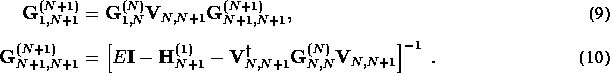
The Green's function is calculated by using the recursive
method (MacKinnon 1985):
Iterative calculations are performed by successively adding slices to the
end of the bar. This numerical technique has proved very reliable for the
Anderson localization problem (MacKinnon and Kramer 1981, Soukoulis et al. 1982). The initial
conditions reflect the environment into which the wire sample is embedded. The
first
slice of the quantum wire (slice 1) is coupled to the end
(slice 0) of the left hand lead, i.e. to a semi-infinite perfect wire. So the
initial
condition for calculating ( in
Eq. (10)) is given by the diagonal block of the Green's function
(
in
Eq. (10)) is given by the diagonal block of the Green's function
( )
at the end of a perfect bar that extends from to 0
(see MacKinnon 1985):
)
at the end of a perfect bar that extends from to 0
(see MacKinnon 1985):
Similarly for the right hand lead:
where  is the self-energy matrix,
which helps us to couple the right hand lead to the other end of conductor.
The effect of adding the whole right hand lead can be represented by the
Hamiltonian:
is the self-energy matrix,
which helps us to couple the right hand lead to the other end of conductor.
The effect of adding the whole right hand lead can be represented by the
Hamiltonian:

in the final iteration of Eq. (10). Iterations of
Eq. (9) for  begin with the unit matrix.
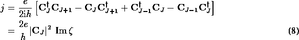
The formulation (2) can be further simplified.
If  is substituted by Eq. (3)
and since the same eigenproblem (5) describes both
left-going and right-going solutions, we get our final result:
is substituted by Eq. (3)
and since the same eigenproblem (5) describes both
left-going and right-going solutions, we get our final result:
Note that the result is not affected by the normalization of  .
This formulation for easily yields transmission probabilities for
the case of a perfect wire of length between two perfect leads of
the same cross-section:
.
This formulation for easily yields transmission probabilities for
the case of a perfect wire of length between two perfect leads of
the same cross-section:
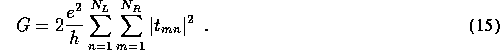
The conductance  , given by the two-terminal Landauer formula
(Landauer 1957, Fisher and Lee 1981), for spin-degenerate states is:
, given by the two-terminal Landauer formula
(Landauer 1957, Fisher and Lee 1981), for spin-degenerate states is:
The summations run over the open channels, of which there are  in the
left lead, and
in the
left lead, and  in the right lead.
The conductance fluctuations are quantified by the square root of the variance
where  denotes averaging over an ensemble of
samples, with different realizations of disorder. In our calculations all the
quantum wires have a hard wall confining potential. Also for the site energy
of islands
denotes averaging over an ensemble of
samples, with different realizations of disorder. In our calculations all the
quantum wires have a hard wall confining potential. Also for the site energy
of islands  is assumed.
The temperature of
the system is always
is assumed.
The temperature of
the system is always  .
.